| Back to Contents | [2] Next Section >>> |
Evert & Krenn (2003) argue strongly for a relational model of cooccurrences, where the cooccurring words must appear in a specific structural relation (usually a syntactic relation). Examples of relational cooccurrence data are prenominal adjectives and the modified nouns in English and German, as well as verbs and their (nominal) objects. In this model, a list of pair tokens is extracted from the source corpus, each one representing an instance of the chosen structural relation. The components of each pair token are then individually assigned to word types, which may represent a specific surface form (word form types), a set of inflected forms derived from the same stem (lemma types), or a more complex mapping (cf. McEnery & Wilson, 2001, p. 82).
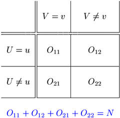
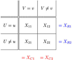
Cooccurrence frequency data are analysed separately for each pair of word types (u,v), called a pair type. Usually, only types that have at least one instance in the source corpus are considered (f ≥ 1). Given a pair type (u,v), the pair tokens extracted from the source corpus are classified into the four cells of a contingency table, depending on whether the first component of the token belongs to type u and whether the second component belongs to type v. These conditions are written U = u and V = v in the contingency table shown below.
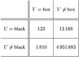
The cell counts O11, ..., O22 of the contingency table are called the observed frequencies of the pair type (u,v). They add up to the total number of pair tokens, called the sample size N. The contingency table below shows the observed frequencies of the adjective-noun pair type (black,box) in the British National Corpus.
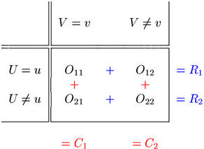
The row totals R1, R2 and column totals C1, C2 often play an important role in the analysis of frequency data. They are referred to as marginal frequencies, being written in the margins of the table. R1 is the marginal frequency of u, i.e. the number of pair tokens whose first component belongs to type u. Similarly, C1 is the marginal frequency of v. O11, the number of cooccurrences, is also called the joint frequency of the pair type (u,v).
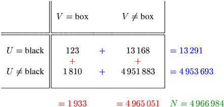
The contingency table below shows the row and column totals of (black,box) in the British National Corpus. From this table, we can see that the joint frequency of this pair type is f = O11= 123. The marginal frequencies are f1 = R1 = 13,291 (13,291 pair tokens of the form (black,*)) and f2 = C1 = 1,933 (1,933 pair tokens of the form (*,box)). The full sample consists of N = 4,966,984 adjective-noun pair tokens extracted from the British National Corpus.
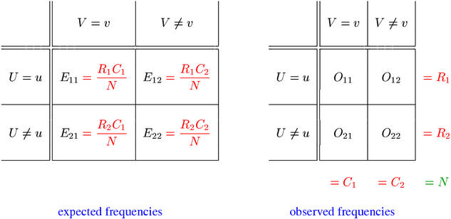
The statistical interpretation of cooccurrence data is based on a random sample model, which assumes that the observed pair tokens are drawn randomly from an infinite population (so that the much simpler equations for sampling with replacement can be used). Such an infinite population can be described as a set of (pair) types and their relative frequencies in the population, which are the parameters of the model. The random selection of a single pair token is modelled by two random variables U and V that represent the component types of the selected token. A sample of N pair tokens is modelled by N independent pairs of random variables Um and Vm, whose distributions are identical to those of the prototypes U and V. Just as with the observed corpus data, the frequency information for a given pair type (u,v) is collected in a contingency table of random variables X11, ..., X22:
X11 is the number of m for which Um = u and Vm = v etc.(1) The marginal frequencies are also random variables, written as XR1, XR2, XC1, and XC2. This contingency table contains all relevant information that a random sample can provide about the pair type (u,v) (formally speaking, it is a sufficient statistic).(2) The contingency table of random variables represents a potential outcome of the sample. The probability of a particular outcome, i.e. a contingency table with cell values k11, ..., k22, is given by the multinomial sampling distribution(3) of (u,v):

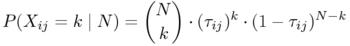
Each random variable Xij has a binomial distribution by itself, so the probability of an outcome with Xij = k (regardless of the other cell values) is
The sampling distribution is determined by the probability parameters τ11, ..., τ22 of (u,v), which can be defined in terms of the prototype variables U and V.
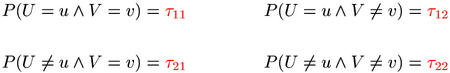
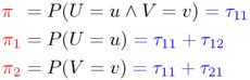
Only three of the four probability parameters, which must add up to one (τ11 + τ12 + τ21 + τ22 = 1) are free parameters. Therefore, it is more common to use an equivalent set of three parameters, given by the equations below. π is the probability that a randomly selected pair token belongs to the pair type (u,v), π1 is the probability that its first component type is u, and π2 that of v being the second component type.
The statistical association between the components u and v of a pair type is a property of its probability parameters (i.e. a population property of the statistical model). Consequently, a main goal of the statistical analysis of cooccurrence data is to make inferences about the population parameters from the observed data. The tables below schematise this comparison between probability parameters and observed frequencies.
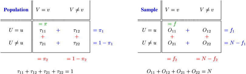
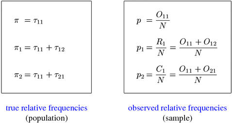
The simplest form of inference are direct ("point") estimates for the probability parameters, which are known as maximum-likelihood estimates (MLE).(4) MLEs for π, π1, and π2 are given by the relative joint and marginal frequencies p, p1, and p2 as shown below.
Unfortunately, the sampling error (i.e. the difference between the true value of a parameter and its estimate) can become quite substantial, especially when the observed frequencies are small. A more responsible approach to statistical inference compares the observed contingency table with the sampling distribution, given some hypothesis about the parameter values. When the observed data correspond to an unlikely outcome of the sample, the null hypothesis is rejected. This procedure is called a statistical hypothesis test. The same approach can also be used to obtain confidence interval estimates for the true values of population parameters.
A fundamental issue in the theory of hypothesis tests is the precise definition of which outcomes should be considered "unlikely". There is no simple answer to this question, which has led to much controversy about the appropriate choice of test for contingency tables.
It is quite obvious that the amount of association between the components of a pair type (u,v) depends in some way on all three probability parameters. However, it is not clear exactly how their values should be combined to obtain a coefficient of association strength as a quantitative measure. Intuitively, a larger value of π indicates stronger association, while larger values of π1 and π2 indicate weaker association. The most straightforward combination is the mu-value coefficient, μ = π ⁄ π1 π2. The less intuitive odds ratio coefficient, θ = τ11 τ22 ⁄ τ12 τ21, is widely used because of its convenient mathematical properties (cf. Agresti, 1990, Ch. 2). Many association measures compute maximum-likelihood or confidence interval estimates for μ, θ, or one of various other coefficients of association strength. I refer to these measures as the degree of association group (see Section 5 & Section 6).
While it is not clear how to measure association strength accurately, there is a well-defined concept for the complete absence of association: statistical independence. When a pair type (u,v) has no association, the events {U = u} and {V = v} must be independent, which leads to the null hypothesis of independence H0 below.
The null hypothesis of independence stipulates a relation between the probability parameters (namely, π = π1 π2), but the parameter values are not completely fixed, and neither is the sampling distribution. The mathematical analysis is greatly simplified (and often made possible in the first place) when H0 is reduced to a point hypothesis by inserting maximum-likelihood estimates for the "nuisance" parameters π1 and π2.(5) Most statistical independence tests for contingency tables are based on this point hypothesis.
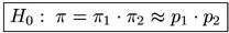
The expectations Eij = E[Xij] of the contingency table cells under the point null hypothesis of independence can easily be computed from the observed row and column totals (shown in the left panel below). I refer to E11, ..., E22 as expected frequencies, but they must not be confused with the expected values of the joint and marginal frequencies given the true population parameters (which may or may not satisfy H0, and will almost certainly not satisfy the point null hypothesis). Hypothesis tests that are based on the point null hypothesis can be understood as a comparison of the contingency tables of expected and observed frequencies, as schematised below.
Forming the second major group of association measures, the significance of association measures use the amount of evidence against the null hypothesis of independence as an association score (see Sections 2, 3 & 4). This amount can be quantified by the likelihood of the observed data (Section 2) or by the p-value of a statistical hypothesis tests (Section 3). Both values are probabilities in the range [0,1] with smaller values indicating more evidence against H0. In order to satisfy the convention that high scores should stand for strong association, the negative base 10 logarithm of the likelihood or p-value is used as an association score (so that e.g. the customary significance level of .001 corresponds to a score of 3.0). Asymptotic hypothesis tests compute an approximate p-value from an intermediate test statistic. This test statistic is often used instead of the p-value as an association score, which simplifies the mathematics considerably (Section 4). However, the latter has the advantage that p-values can directly be compared between different measures from the significance of association group.
| Back to Contents | [2] Next Section >>> |