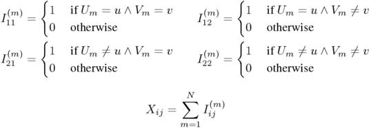
1 Formally, the variables Xij can be defined as sums over indicator variables:
2 Intuitively, the particular arrangement of the pair tokens in the sample cannot provide any meaningful information, since it is presupposed to be random. In particular, all reorderings of the sample must be equally likely. It is therefore sufficient to consider the total (co)occurrence frequencies. In fact, a sufficient statistic is already given by three of the variables in a contingency table (e.g. the joint frequency X11 and the first row and column totals XR1 and XC1) because the four cells must add up to the sample size: X11 + X12 + X21 + X22 = N.
3 Formally, the sampling distribution is the joint probability distribution of the random variables X11, ..., X22.
4 The name maximum-likelihood estimates derives from the fact that the estimated values maximise the probability (or likelihood) of the observed contingency table among the set of all possible parameter values.
5 Precisely speaking, the point null hypothesis consists of three conditions: π1 = p1, π2 = p2, and π = p1 p2. Although p1 and p2 are random variables, they are treated as constants in the statistical model, which are set to the values computed from the observed data. Hypothesis tests based on the point null hypothesis thus effectively ignore the sampling error of p1 and p2.
1 This likelihood is the probability of an outcome where X11 equals the observed value O11, while the values of X12, X21, and X22 are unspecified. Note that the observed marginal frequencies still have some effect through their influence on the point null hypothesis.
1
Try the command phyper(99, 1000, 999000, 1000, lower=F), which
computes the Fisher score for a contingency table with
O11 = 100, R1 = C1 = 1,000,
and N = 1,000,000. At least on versions up to R-1.9.0 running under Linux/i386,
the result is a negative p-value (P < 0)!
1 In earlier days, this task involved enormous tomes of statistical tables where p-values for many known distributions were tabulated. Back then, without the help of desktop computers, it was impossible to carry out exact hypothesis tests except for the case of very small samples. Such practical considerations were an important reason for the concentration on asymptotic (rather than exact) hypothesis tests during the first half of the 19th century.
2 For instance, common sense dictates that in those cases where a contingency table A is clearly less consistent with the null hypothesis than a table B, the test statistic should assume a greater value for A than for B. In many other cases, where the desired result of the comparison is not obvious, the definition of the test statistic is essentially an intuitive choice.
3 An equivalence proof for the three different versions of the chi-squared measure can be based on the fact that the identity (O11 - E11)2 = (O12 - E12)2 = (O21 - E21)2 = (O22 - E22)2 holds for any contingency table.
4 The number of degrees of freedom is given by the dimension of the parameter space minus the dimension of the null hypothesis (which is formally a subset of the parameter space). In the case of coocurrence data, the former has dimension 3 (with free parameters π, π1, π2), while the latter has dimension 2 (with π1, π2 as free parameters, and π determined by H0). Therefore, the limiting χ2 distribution of the likelihood ratio statistic has one degree of freedom.
1 In particular, odds-ratio does not make any distinction between contingency tables where either O12 = 0 or O21 = 0 (because they are assigned the same infinite score). After discounting, odds-ratiodisc assigns higher scores to tables where both non-diagonal cells are empty (O12 = O21 = 0) rather than just one, and it takes the cooccurrence frequency O11 into account.
2 In the same paper, the authors also argue in favour of point estimates, which they interpret as descriptive rather than inferential measures. They state that descriptive statistics are more appropriate when it is feasible to analyse a population exhaustively (which they imply to be the case for the very large corpora that are available today). Interestingly, this argument is followed by an empirical evaluation of the MS measure (as an example of a descriptive measure) on a subset of the Wall Street Journal.
3 Let g be the Dice score for a given contingency table. Then the Jaccard score h for the same table is given by the equation h = g &frasl (2 - g).
1 Let g be the local-MI score for a given pair type (u,v), and let h be the score of the Poisson-Stirling measure. Then the following equality holds: h = g - O11.
1 Let g be the gmean association score for a pair type (u,v). Then the score h of the MI2 measure is given by h = log(g2) + log N, which is a monotonic transformation (for a fixed sample of size N).